Tutorial

Assuming that you have Aurora already installed on your system, we’re now ready to move forward. Some basic Aurora functionality is demonstrated in the examples package directory, where users may find a number of useful scripts. Here, we go through some of the same examples and methods.

Core impurity transport simulations

If Aurora is correctly installed, you should be able to do:

import aurora

and then load a default namelist for impurity transport forward modeling:

namelist = aurora.load_default_namelist()

Note that you can always look at where this function is defined in the package by using, e.g.:

aurora.load_default_namelist.__module__

Once you have loaded the default namelist, have a look at the namelist dictionary. It contains a number of parameters that are needed for Aurora runs. Some of them, like the name of the device, are only important if automatic fetching of the EFIT equilibrium through MDSplus is required, or else it can be ignored (leaving it to its default value). Most of the parameter names should be fairly self-descriptive. Please refer to docstrings throughout the code documentation.

Aurora leverages the omfit_classes package to interface with MDS+, EFIT, and a number of other codes. Thanks to this, users can focus more on their applications of interest, and less on re-inventing the wheel to write code that the OMFIT Team has kindly made public! To follow the rest of this tutorial, do:

from omfit_classes import omfit_eqdsk, omfit_gapy

Next, we read in a magnetic equilibrium. You can find an example from a C-Mod discharge in the examples directory:

geqdsk = omfit_eqdsk.OMFITgeqdsk('example.gfile')

The output geqdsk dictionary contains the contents of the EFIT geqdsk file, with additional processing done by the omfit_classes package for flux surfaces. Only some of the dictionary fields are used; refer to the grids_utils methods for details. The geqdsk dictionary is used to create a mapping between the rhop grid (square root of normalized poloidal flux) and a rvol grid, defined by the normalized volume of each flux surface. Aurora, like STRAHL, runs its simulations on the rvol grid.

We next need to read in some kinetic profiles, for example from an input.gacode file (available in the examples directory):

inputgacode = omfit_gapy.OMFITgacode('example.input.gacode')

Other file formats (e.g. plasma statefiles, TRANSP outputs, etc.) may also be read with omfit_gapy or other OMFIT-distributed packages. It is however not important to Aurora how the users get kinetic profiles: all that matters is that they are stored in the namelist[‘kin_prof’] dictionary. To set up time-independent kinetic profiles we can use:

kp = namelist['kin_profs']
kp['Te']['rhop'] = kp['ne']['rhop'] = np.sqrt(inputgacode['polflux']/inputgacode['polflux'][-1])
kp['ne']['vals'] = inputgacode['ne']*1e13    # 1e19 m^-3 --> cm^-3
kp['Te']['vals'] = inputgacode['Te']*1e3     # keV --> eV

Note that both electron density (ne) and temperature (Te) must be saved on a rhop grid. This grid is internally used by Aurora to map to the rvol grid. Also note that, unless otherwise stated, Aurora inputs are always in CGS units, i.e. all spatial quantities are given in \(cm\)!! (the extra exclamation mark is there for a good reason…).

Next, we specify the ion species that we want to simulate. We can simply do:

imp = namelist['imp'] = 'Ar'

and Aurora will internally find ADAS data for that ion (assuming that this is one of the common ones for fusion modeling). The namelist also contains information on what kind of source of impurities we need to simulate; here we are going to select a constant source (starting at t=0) of \(10^{24}\) particles/second.:

namelist['source_type'] = 'const'
namelist['source_rate'] = 1e24

Time dependent time histories of the impurity source may however be given by selecting namelist[‘source_type’]=”step” (for a series of step functions), “synth_LBO” (for an analytic function resembling a laser-blow-off (LBO) time history) or “file” (to load a detailed function from a file). Refer to the get_source_time_history() method for more details.

Assuming that we’re happy with all the inputs in the namelist at this point (many more could be changed!), we can now go ahead and set up our Aurora simulation::

asim = aurora.aurora_sim(namelist, geqdsk=geqdsk)

The aurora_sim class creates a Python object with spatial and temporal grids, kinetic profiles, atomic rates and all other inputs to the forward model. Aurora uses a diffusive-convective model for particle fluxes, so we need to specify diffusion (D) and convection (V) coefficients next::

D_z = 1e4 * np.ones(len(asim.rvol_grid))  # cm^2/s
V_z = -2e2 * np.ones(len(asim.rvol_grid)) # cm/s

Here we have made use of the rvol_grid attribute of the asim object, whose name is self-explanatory. This grid has a 1-to-1 correspondence with asim.rhop_grid. In the lines above we have created flat profiles of \(D=10^4 cm^2/s\) and \(V=-2\times 10^2 cm/s\), defined on our simulation grids. D’s and V’s could in principle (and, very often, in practice) be defined with more dimensions to represent a time-dependence and also different values for different charge states. Unless specifed otherwise, Aurora assumes all points of the time grid (now stored in asim.time_grid) and all charge states to have the same D and V. See the aurora.core.run_aurora() method for details on how to speficy further dependencies.

At this point, we are ready to run an Aurora simulation, with:

out = asim.run_aurora(D_z, V_z)

Blazing fast! Depending on how many time and radial points you have requested (a few hundreds by default), how many charge states you are simulating, etc., a simulation could take as little as <50 ms, which is significantly faster than other code, as far as we know. If you add use_julia=True to the aurora.core.run_aurora() call the run will be even faster; wear your seatbelt!

You can easily check the quality of particle conservation in the various reservoirs by using:

reservoirs = asim.check_conservation()

which will show the results in full detail. The reservoirs output list contains information about how many particles are in the plasma, in the wall reservoir, in the pump, etc.. Refer to the aurora.core.run_aurora() docstring for details.

A plot is worth a thousand words, so let’s make one for the charge state densities::

nz = out[0]  # charge state densities are stored first in the output of the run_aurora method
aurora.slider_plot(asim.rvol_grid, asim.time_out, nz.t.transpose(1,0,2),
                   xlabel=r'$r_V$ [cm]', ylabel='time [s]', zlabel='Total radiation [A.U.]',
                   labels=[str(i) for i in np.arange(0,nz.shape[1])],
                   plot_sum=True, x_line=asim.rvol_lcfs )

You should get a slider showing a result like the following:

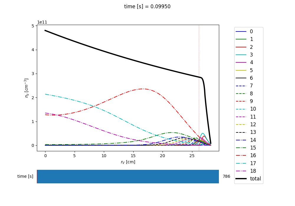
Example of charge state density profiles at the end of an Aurora Ar simulation

Use the slider to go over time, as you look at the distributions over radius of all the charge states. It would be really great if you could just save this type of time- and spatially-dependent visualization to a video-format, right? That couldn’t be easier, using the animate_aurora() function::

aurora.animate_aurora(asim.rhop_grid, asim.time_out, nz.transpose(1,0,2),
                      xlabel=r'$\rho_p$', ylabel='t={:.4f} [s]', zlabel=r'$n_z$ [A.U.]',
                      labels=[str(i) for i in np.arange(0,nz.shape[1])],
                      plot_sum=True, save_filename='aurora_anim')

After running this, a .mp4 file with the name “aurora_anim.mp4” will be saved locally.

Radiation predictions

Once a set of charge state densities has been obtained, it is simple to compute radiation terms in Aurora. For example, using the results from the Aurora run in Running Aurora simulations, one can then run:

asim.rad = aurora.compute_rad(imp, nz.transpose(2,1,0), asim.ne, asim.Te, prad_flag=True)

The documentation on compute_rad() gives details on input array dimensions and various flags that may be turned on. In the case above, we simply indicated the ion number (imp), and provided charge state densities (with dimensions of time, charge state and space), electron density and temperature (dimensions of time and space). We then explicitely indicated prad_flag=True, which means that unfiltered “effective” radiation terms (line radiation and continuum radiation) should be computed. Bremsstrahlung is also estimated using an interpolation formula that is independent of ADAS data and can be found in asim.rad[‘brems’]. However, note that bremsstrahlung is already included in asim.rad[‘cont_rad’], which also includes other terms including continuum recombination using ADAS data. It can be useful to compare the bremsstrahlung calculation in asim.rad[‘brems’] with asim.rad[‘cont_rad’], but we recommend that users rely on the full continuum prediction for total power estimations.

Other possible flags of the compute_rad() function include:

1. sxr_flag: if True, compute line and continuum radiation in the SXR range using the ADAS “pls” and “prs” files. Bremsstrahlung is also separately computed using the ADAS “pbs” files.

2. thermal_cx_rad_flag: if True, the code checks for inputs n0 (atomic H/D/T neutral density) and Ti (ion temperature) and computes line power due to charge transfer from thermal background neutrals and impurities.

3. spectral_brem_flag: if True, use the ADAS “brs” files to compute bremsstrahlung at a wavelength specified by the chosen file.

All of the radiation flags are False by default.

ADAS files for all calculations are taken by default from the list of files indicated in adas_files_dict() function, but may be replaced by specifying the adas_files dictionary argument to compute_rad().

Results from compute_rad() are collected in a dictionary (named “rad” above and added as an attribute to the “asim” object, for convenience) with clear keys, described in the function documentation. To get a quick plot of the radiation profiles, e.g. for line radiation from all simulated charge states, one can do:

aurora.slider_plot(asim.rvol_grid, asim.time_out, asim.rad['line_rad'].transpose(1,2,0),
                   xlabel=r'$r_V$ [cm]', ylabel='time [s]', zlabel='Total radiation [A.U.]',
                   labels=[str(i) for i in np.arange(0,nz.shape[1])],
                   plot_sum=True, x_line=asim.rvol_lcfs)

This will give you a slider again, showing figures like this:

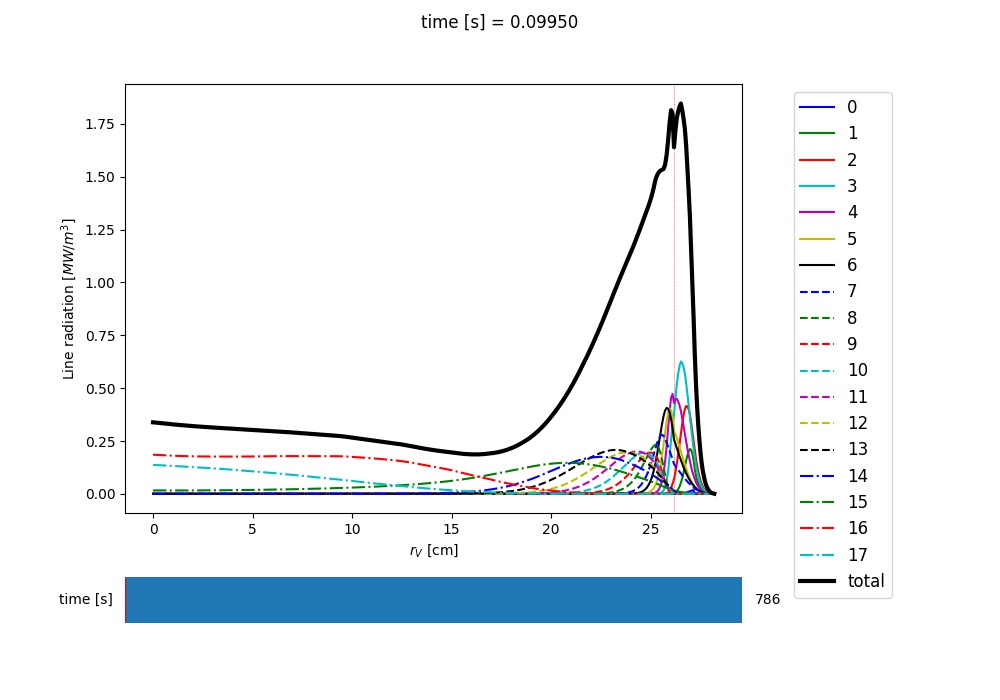
Example of line radiation at the end of an Aurora Ar simulation

Aurora’s radiation modeling capabilities may also be useful when assessing total power radiation for integrated modeling. The radiation_model() function allows one to easily obtain the most important radiation terms at a single time slice, both as power densities (units of \(MW/cm^{-3}\)) and absolute power (units of \(MW\)). To obtain the latter form, we need to integrate over flux surface volumes. To do so, we make use of the geqdsk dictionary obtained via:

geqdsk = omfit_eqdsk.OMFITgeqdsk('example.gfile')

We then pass that to radiation_model(), together with the impurity atomic symbol (imp), the rhop grid array, electron density (ne_cm3) and temperature (Te_eV), and optionally also background neutral densities to include thermal charge exchange::

res = aurora.radiation_model(imp,rhop,ne_cm3,Te_eV, geqdsk,
                             n0_cm3=None, frac=0.005, plot=True)

Here we specified the impurity densities as a simple fraction of the electron density profile, by specifying the frac argument. This is obviously a simplifying assumption, effectively stating that the total impurity density profile should have a maximum amplitude of frac (in the case above, set to 0.005) and a profile shape (corresponding to a profile of V/D) that is identical to the one of the \(n_e\) profile. This may be convenient for parameter scans in the design process of future devices, but is by no means a correct assumption. If we’d rather calculate the total radiated power from a specific set of impurity charge state profiles (e.g. from an Aurora simulation), we can do:

res = aurora.radiation_model(imp,rhop,ne_cm3,Te_eV, geqdsk,
                             n0_cm3=None, nz_cm3=nz_cm3, plot=True)

where we specified the charge state densities (dimensions of space, charge state) at a single time. Since we specified plot=True, a number of useful radiation profiles should be displayed.

Of course, one can also estimate radiation from the main ions. To do this, we first want to estimate the main ion density, using:

ni_cm3 = aurora.get_main_ion_dens(ne_cm3, ions)

with ions being a dictionary of the form:

ions = {'C': nC_cm3, 'Ne': nNe_cm3}   # (time,charge state,space)

with a number of impurity charge state densities with dimensions of (time,charge state,space). The get_main_ion_dens() function subtracts each of these densities (times the Z of each charge state) from the electron density to obtain a main ion density estimate based on quasineutrality. Before we move forward, we need to add a neutral stage density for the main ion species, e.g. using:

niz_cm3 = np.vstack((n0_cm3[None,:],ni_cm3)).T

such that the niz_cm3 output is a 2D array of dimensions (charge states, radii).

To estimate main ion radiation we can now do:

res_mainion = aurora.radiation_model('H',rhop,ne_cm3,Te_eV, vol, nz_cm3 = niz_cm3, plot=True)

(Note that the atomic data does not discriminate between hydrogen isotopes) In the call above, the neutral density has been included in niz_cm3, but note that (1) there is no radiation due to charge exchange between deuterium neutrals and deuterium ions, since they are indistinguishable, and (2) we did not attempt to include the effect of charge exchange on deuterium fractional abundances because n0_cm3 (included in niz_cm3 already fully specifies fractional abundances for main ions).

Zeff contributions

Following an Aurora run, one may be interested in what is the contribution of the simulated impurity to the total effective charge of the plasma. The calc_Zeff() method allows one to quickly compute this by running:

asim.calc_Zeff()

This makes use of the electron density profiles (as a function of space and time), stored in the “asim” object, and keeps Zeff contributions separate for each charge state. They can of course be plotted with slider_plot()::

aurora.slider_plot(asim.rvol_grid, asim.time_out, asim.delta_Zeff.transpose(1,0,2),
                   xlabel=r'$r_V$ [cm]', ylabel='time [s]', zlabel=r'$\Delta$ $Z_{eff}$',
                   labels=[str(i) for i in np.arange(0,nz.shape[1])],
                   plot_sum=True,x_line=asim.rvol_lcfs)

You should get something that looks like this:

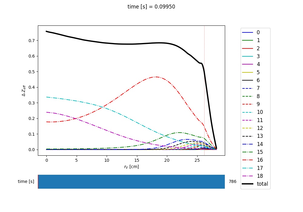
Example of Z-effective contributions at the end of an Aurora Ar simulation

Ionization equilibrium

It may be useful to compare and contrast the charge state distributions obtained from an Aurora run with the distributions predicted by pure ionization equilibium, i.e. by atomic physics only, with no trasport. To do this, we only need some kinetic profiles, which for this example we will load from the sample input.gacode file available in the “examples” directory:

import omfit_gapy
inputgacode = omfit_gapy.OMFITgacode('example.input.gacode')

Recall that Aurora generally uses CGS units, so we need to convert electron densities to \(cm^{-3}\) and electron temperatures to \(eV\):

rhop = np.sqrt(inputgacode['polflux']/inputgacode['polflux'][-1])
ne_vals = inputgacode['ne']*1e13 # 1e19 m^-3 --> cm^-3
Te_vals = inputgacode['Te']*1e3  # keV --> eV

Here we also defined a rhop grid from the poloidal flux values in the inputgacode dictionary. We can then use the get_atom_data() function to read atomic effective ionization (“scd”) and recombination (“acd”) from the default ADAS files listed in adas_files_dict(). In this example, we are going to focus on calcium ions:

atom_data = aurora.get_atom_data('Ca',['scd','acd'])

In ionization equilibrium, all ionization and recombination processes will be perfectly balanced. This condition corresponds to specific fractions of each charge state at some locations that we define using arrays of electron density and temperature. We can compute fractional abundances and plot results using:

Te, fz = aurora.get_frac_abundances(atom_data, ne_vals, Te_vals, rho=rhop, plot=True)

The get_frac_abundances() function returns the log-10 of the electron temperature on the same grid as the fractional abundances, given by the fz parameter (dimensions: space, charge state). This same function can be used to both compute radiation profiles of fractional abundances or to compute fractional abundances as a function of scanned parameters ne and/or Te.

Additionally, the function get_atomic_relax_time() allows one to obtain the relaxation time of the ionization equilibrium for a given species, which permits an assessment of the time scales for atomic vs transport effects. The effect of transport can be mimicked by passing a tau_s parameter, representing a typical (global) particle residence time. This capability can be used, for example, to explore how sensitive the ionization balance is to transport, but it can of course only provide a very approximate assessment.

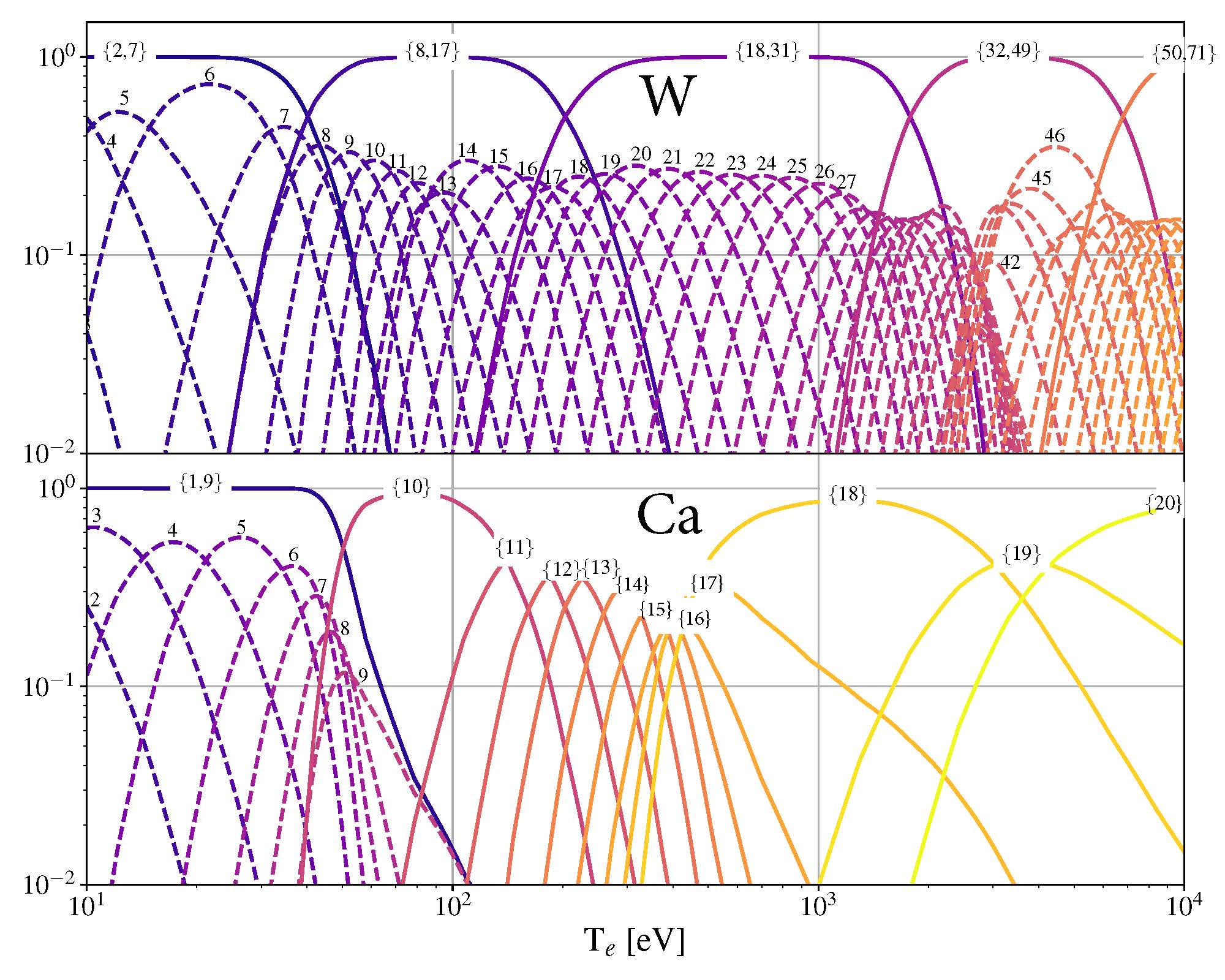
Ionization equilibria of W and Ca (dashed lines), also showing some choices of charge state bundling (superstaging) for both species.

The figure above shows examples of ionization equilibria for W and Ca as a function of electron temperature. Dashed lines here show the complete/standard result, whereas the continuous lines show examples of charge state bundling (superstaging), using arbitrarily-chosen partitions. Superstaging is an extremely useful and interesting technique to reduce the computational complexity of medium- and high-Z ions, since often the cost of simulations scales linearly (as in Aurora), or worse, with the number of charge states (Z). You can read more about superstaging in the paper F Sciortino et al 2021 Plasma Phys. Control. Fusion 63 112001.

Atomic spectra

If you have atomic data files containing photon emissivity coefficients (PECs) in ADF15 format, you can use Aurora to combine them and see what the overall spectrum might look like. Let’s say you want to look at the \(K_\alpha\) spectrum of Ca at a specific electron density of \(10^{14}\) \(cm^{-3}\) and temperature of 1 keV. Let’s begin with a single ADF15 file located at the following path:

filepath_he='~/pec#ca18.dat'

The simplest way to check what the spectrum may look like is to weigh contributions from different charge states according to their fractional abundances at ionization equilibrium. Aurora allows you to get the fractional abundances with just a couple of lines:

ion = 'Ca'
ne_cm3 = 1e14
Te_eV = 1e3
atom_data = aurora.get_atom_data(ion,['scd','acd'])
Te, fz = aurora.get_frac_abundances(atom_data, np.array([ne_cm3,]), np.array([Te_eV,]), plot=False)

You can now use the aurora.get_local_spectrum function to read all the lines in each ADF15 file and broaden them according to some ion temperature (which could be dictated by broadening mechanisms other than Doppler effects, in principle). For our example, one can do:

# He-like state
out= aurora.get_local_spectrum(filepath_he, ion, ne_cm3, Te_eV, n0_cm3=0.0,
                             ion_exc_rec_dens=[fz[0,-4], fz[0,-3], fz[0,-2]], # Li-like, He-like, H-like
                             dlam_A = 0.0, plot_spec_tot=False, no_leg=True,
                             plot_all_lines=True, ax=None)
wave_final_he, spec_ion_he, spec_exc_he, spec_rec_he, spec_dr_he, spec_cx_he, ax = out

By changing the dlam_A parameter, you can also add a wavelength shift (e.g. from the Doppler effect). The ion_exc_rec_dens parameter allows specification of fractional abundances for the charge stages of interest. To be quite general, in the lines above we have included contributions to the spectrum from ionizing, excited and recombining PEC components. By passing an ax argument one can also specify which matplotlib axes are used for plotting.

By repeating the same operations using several ADF15 files, one can overplot contributions to the spectrum from several charge states. As an example, the figure below shows the K-alpha spectrum of Ca, with contributions from Li-like, He-like and H-like Ca, evaluated at 1 keV and \(10^{20}\) \(cm^{-3}\).

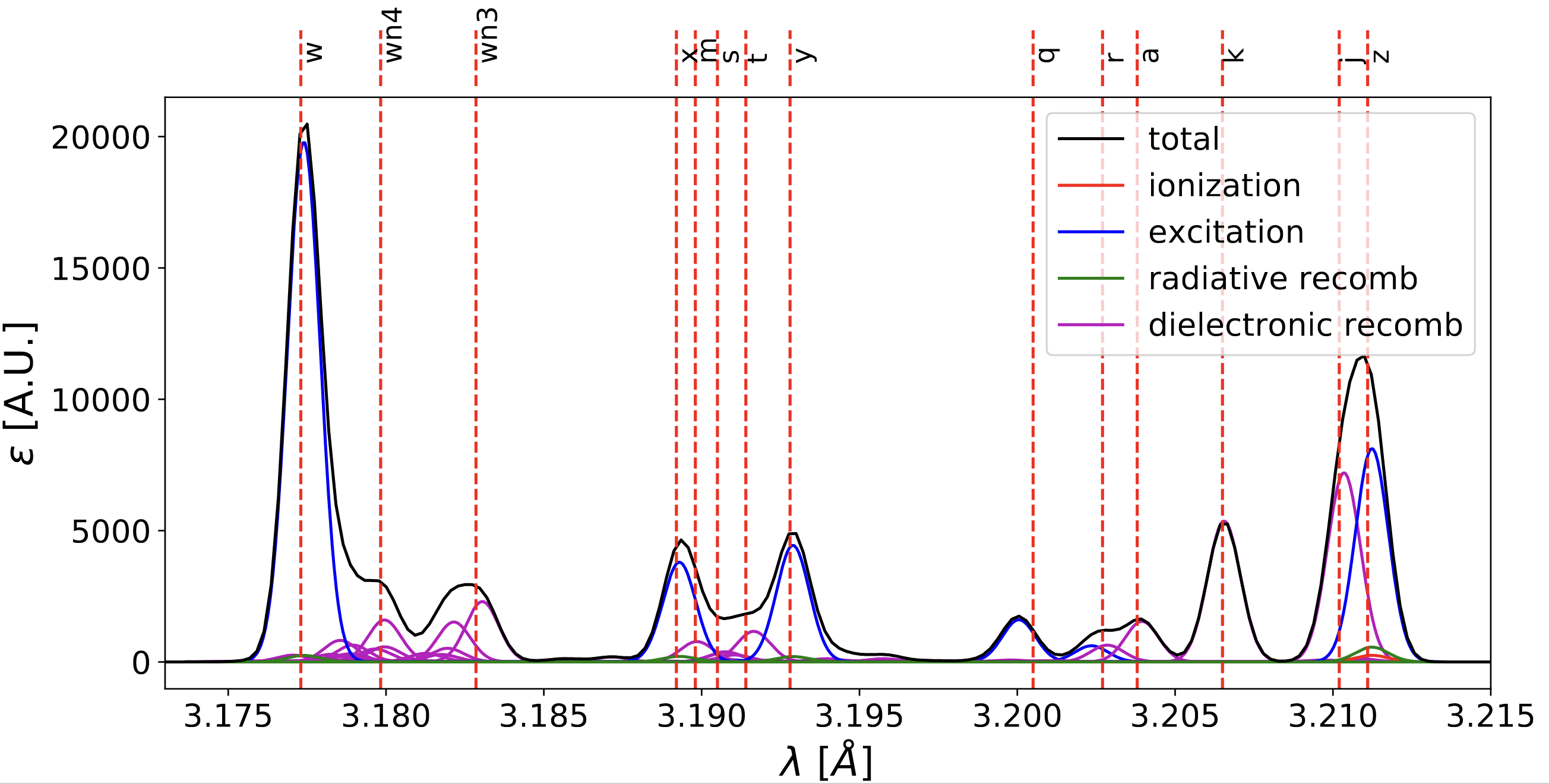
Example of high-resolution K-alpha spectrum of Ca

If you just want to plot where atomic lines are expected to be and how intense their PECs are at specific plasma conditions, you can also use the simpler aurora.adf15_line_identification function. This can be called as:

aurora.adf15_line_identification(pec_files, Te_eV=Te_eV, ne_cm3=ne_cm3, mult=mult)

and can be used to plot something like this:

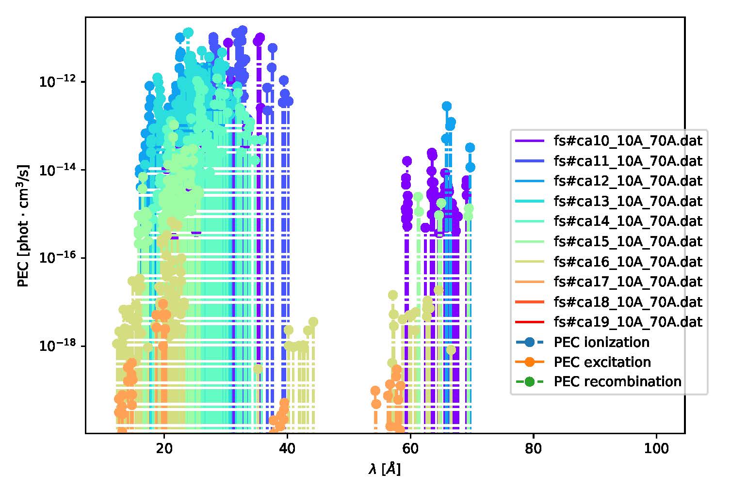
Example of Ca spectrum overview combining several PEC files

A&M data from AMJUEL/HYDHEL

Aurora allows one to load and process atomic and molecular (A&M) rates collected in the form of polynomial fits in the AMJUEL and HYDHEL databases, publicly released as part of the EIRENE code. These rates are partly redundant and partly complement those provided by ADAS.

The following code illustrates how one may evaluate A&M components of the Balmer lines of deuterium:

import os, copy
import numpy as np
import matplotlib.pylab as plt

plt.ion()
import sys

# Make sure that package home is added to sys.path
sys.path.append("../")
import aurora

rdb = aurora.amdata.reactions_database()


RR_alpha = [
    "AMJUEL,12,2_1_5a",  # H(3)/H
    "AMJUEL,12,2_1_8a",  # H(3)/H+
    "AMJUEL,12,2_2_5a",  # H(3)/H2
    "AMJUEL,12,2_2_14a",  # H(3)/H2+
    "AMJUEL,12,2_0c",  # H2+/H2
    "AMJUEL,12,7_2a",  # H(3)/H-
    "AMJUEL,11,7_0a",  # H-/H2
    "AMJUEL,12,2_2_15a",  # H(3)/Hll3+    # not used
    "AMJUEL,11,4_0a",  # H3+/H2/H2+/ne  # not used
]

# Lyman series spontaneous emission coeffs for n=2 to 1, 3 to 1, ... 16 to 1
A_lyman = [
    4.699e8,
    5.575e7,
    1.278e7,
    4.125e6,
    1.644e6,
    7.568e5,
    3.869e5,
    2.143e5,
    1.263e5,
    7.834e4,
    5.066e4,
    3.393e4,
    2.341e4,
    1.657e4,
    1.200e4,
]

# Balmer series spontaneous emission coeffs for n=3 to 2, 4 to 2, ... 17 to 2
A_balmer = [
    4.41e7,
    8.42e6,
    2.53e6,
    9.732e5,
    4.389e5,
    2.215e5,
    1.216e5,
    7.122e4,
    4.397e4,
    2.83e4,
    18288.8,
    12249.1,
    8451.26,
    5981.95,
    4332.13,
]

fig, ax = plt.subplots(2, 1, sharex=True)
ls_list = ["-", "--", "-.", ":"]

nt = 200
lines = ["alpha", "beta", "gamma", "delta"]
rates = np.zeros((len(RR_alpha), nt, len(lines)))

for ii, choice in enumerate(lines):

    ls = ls_list[ii]

    # allow one to read various Balmer-series lines by changing final reaction letter
    sub = {"alpha": "a", "beta": "c", "gamma": "d", "delta": "e"}
    RR = copy.deepcopy(RR_alpha)
    for i in [0, 1, 2, 3, 5, 7]:  # only cross sections specific to Halpha
        RR[i] = "AMJUEL" + RR_alpha[i].split("AMJUEL")[1].replace("a", sub[choice])

    # select Einstein Aki coefficients
    aa = {"alpha": 0, "beta": 1, "gamma": 2, "delta": 3}
    a0 = A_balmer[aa[choice]]

    te = np.linspace(0.2, 10.0, nt)
    ne = np.ones(nt) * 1e19
    ni = np.ones(nt) * 1e19
    nh = np.ones(nt) * 1e19
    nh2 = np.ones(nt) * 1e19

    for j, R in enumerate(RR):
        rdb.select_reaction(R)
        rates[j, :, ii] = rdb.reaction(ne, te)

    c1 = a0 * rates[0, :, ii] * nh
    c2 = a0 * rates[1, :, ii] * ni
    c3 = a0 * rates[2, :, ii] * nh2
    c4 = a0 * rates[3, :, ii] * rates[4, :, ii] * nh2
    c5 = a0 * rates[5, :, ii] * rates[6, :, ii] * nh2
    ct = c1 + c2 + c3 + c4 + c5  # np.ones_like(c1)

    ax[0].plot(te, ct, c="k", ls=ls)
    ax[1].plot(te, c1 / ct, c="b", ls=ls)
    ax[1].plot(te, c2 / ct, c="c", ls=ls)
    ax[1].plot(te, c3 / ct, c="g", ls=ls)
    ax[1].plot(te, c4 / ct, c="r", ls=ls)
    ax[1].plot(te, c5 / ct, c="m", ls=ls)

ax[0].plot([], [], c="k", ls="-", label="alpha")
ax[0].plot([], [], c="k", ls="--", label="beta")
ax[0].plot([], [], c="k", ls="-.", label="gamma")
ax[0].plot([], [], c="k", ls=":", label="delta")
ax[0].legend(loc="best").set_draggable(True)
ax[0].set_yscale("log")
ax[0].set_ylabel("$\epsilon_{tot}$ [ph/m$^{-3}$]")

ax[1].plot([], [], c="b", label="H")
ax[1].plot([], [], c="c", label="H+")
ax[1].plot([], [], c="g", label="H2")
ax[1].plot([], [], c="r", label="H2+")
ax[1].plot([], [], c="m", label="H2-")
ax[1].legend(loc="best").set_draggable(True)
ax[1].set_yscale("log")
ax[1].set_ylim((1e-3, 1e0))
ax[1].set_xlabel("$T_e$ [eV]")
ax[1].set_ylabel("$\epsilon_i/\epsilon_{tot}$")

Working with neutrals

Aurora includes a number of useful functions for neutral modeling, both from the edge of fusion devices (thermal neutrals) and from neutral beams (fast and halo neutrals).

For thermal neutrals, we make use of atomic data from the Collrad collisional-radiative model, part of the DEGAS2 code.

The erh5_file class allows one to parse the erh5.dat file of DEGAS-2 that contains useful information to assess excited state fractions of neutrals in specific kinetic backgrounds. If the erh5.dat file is not available already, Aurora will download it and store it locally within its distribution directory. The data in this file is used for example in the get_exc_state_ratio() function, which given a ground state density of neutrals (N1), some ion and electron densities (ni and ne) and electron temperature (Te), will compute the fraction of neutrals in the principal quantum number m. Keyword arguments can be passed to this function to plot the results. Note that kinetic inputs may be given as a scalar or as a 1D list/array. The plot_exc_ratios() function may also be useful to plot the excited state ratios.

Note that in order to find the photon emissivity coefficient of specific neutral lines, the read_adf15() function may be used. For example, to obtain interpolation functions for neutral H Lyman-alpha emissivity, one can use:

filename = 'pec96#h_pju#h0.dat' # for D Ly-alpha

# fetch file automatically, locally, from AURORA_ADAS_DIR, or directly from the web:
path = aurora.get_adas_file_loc(filename, filetype='adf15')

# load all the transitions in the chosen ADF15 file -- returns a pandas.DataFrame
trs = aurora.read_adf15(path)

# select and plot the Lyman-alpha line at 1215.2 A
tr = trs.loc[(trs['lambda [A]']==1215.2) & (trs['type']=='excit')]
aurora.plot_pec(tr)

This will plot the Lyman-alpha photon emissivity coefficients (both the components due to excitation and recombination) as a function of temperature in eV, as shown in the figures below.

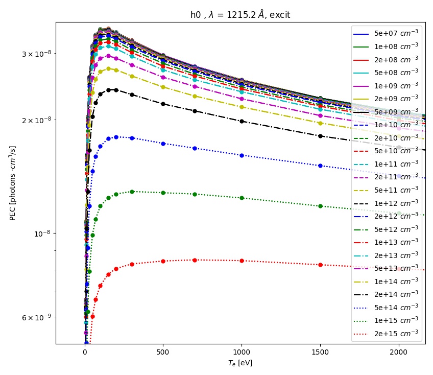
ADAS photon emissivity coefficients for the excitation contribution to the H \(Ly_\alpha\) transition.

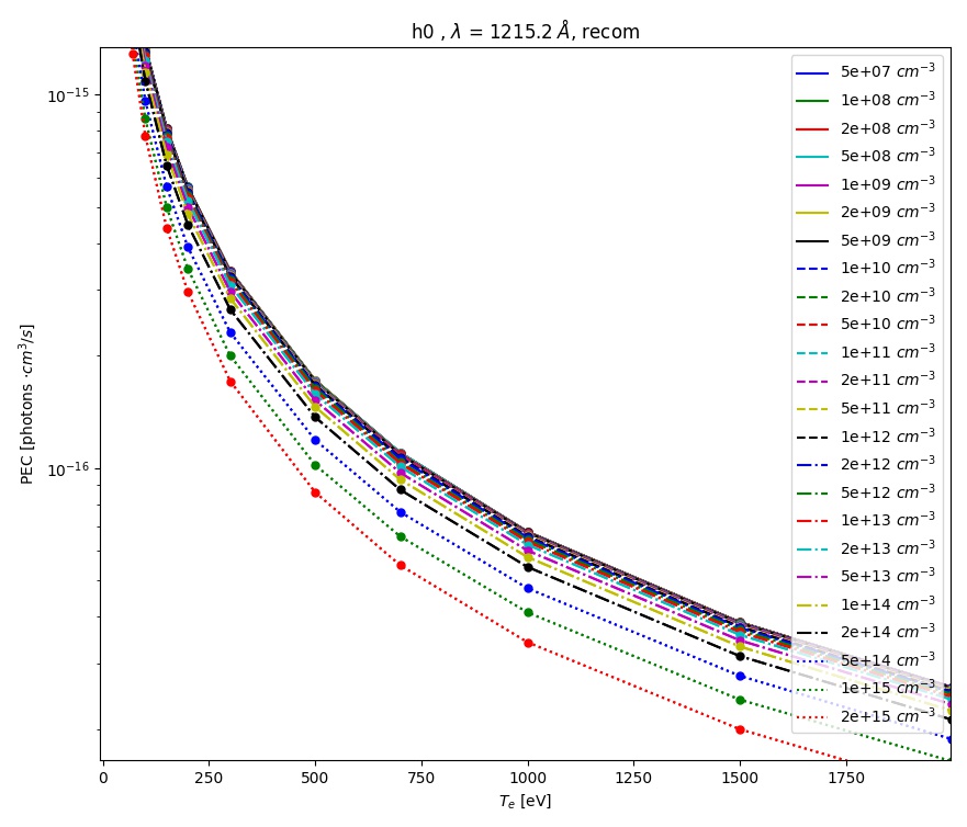
ADAS photon emissivity coefficients for the recombination contribution to the H \(Ly_\alpha\) transition.

Some files (e.g. try pec96#c_pju#c2.dat) may also have charge exchange components. Note that both the inputs and outputs of the read_adf15() function act on log-10 values, i.e. interpolants should be called on log-10 values of \(n_e\) and \(T_e\), and the result of interpolation will only be in units of \(photons \cdot cm^3/s\) after one takes the power of 10 of it.

Analysis routines to work with fast and halo neutrals are also provided in Aurora. Atomic rates for charge exchange of impurities with NBI neutrals are taken from Janev & Smith NF 1993 and can be obtained from js_sigma(), which wraps a number of functions for specific atomic processes. To compute charge exchange rates between NBI neutrals (fast or thermal) and any ions in the plasma, users need to provide a prediction of neutral densities, likely from an external code like FIDASIM.

Neutral densities for each fast ion population (full-,half- and third-energy), multiple halo generations and a few excited states are expected. Refer to the documentation of get_neutrals_fsa() to read about how to provide neutrals on a poloidal cross section so that they may be “flux-surface averaged”.

bt_rate_maxwell_average() shows how beam-thermal Maxwell-averaged rates can be obtained; tt_rate_maxwell_average() shows the equivalent for thermal-thermal Maxwell-averaged rates.

Finally, get_NBI_imp_cxr_q() shows how flux-surface-averaged charge exchnage recombination rates between an impurity ion of charge q with NBI neutrals (all populations, fast and thermal) can be computed for use in Aurora forward modeling. For more details, feel free to contact Francesco Sciortino (sciortino-at-psfc.mit.edu).

Interfacing with SOLPS-ITER

While running SOLPS-ITER is a complex task, reading and processing its results does’t need to be. Aurora offers a convenient Python interface to rapidly load results, set them to convenient data arrays, plot on 1D or 2D grids, etc.

Here’s an example of how you could load a SOLPS-ITER run and create some useful plots:

"""
Script to demonstrate capabilities to load and post-process SOLPS results.
Note that SOLPS output is not distributed with Aurora; so, in order to run this script,
either you are able to access the default AUG SOLPS MDS+ server, or you need
to appropriately modify the script to point to your own SOLPS results.
"""
import numpy as np
import matplotlib.pyplot as plt

plt.ion()
from omfit_classes import omfit_eqdsk
import sys, os
import aurora

# if one wants to load a SOLPS case from MDS+ (defaults for AUG):
so = aurora.solps_case(solps_id=141349)

# alternatively, one may want to load SOLPS results from files on disk:
so2 = aurora.solps_case(
    b2fstate_path="/afs/ipp/home/s/sciof/SOLPS/141349/b2fstate",
    b2fgmtry_path="/afs/ipp/home/s/sciof/SOLPS/141349/b2fgmtry",
)

# plot some important fields
fig, axs = plt.subplots(1, 2, figsize=(10, 6), sharex=True)
ax = axs.flatten()
so.plot2d_b2(so.data("ne"), ax=ax[0], scale="log", label=r"$n_e$ [$m^{-3}$]")
so.plot2d_b2(so.data("te"), ax=ax[1], scale="linear", label=r"$T_e$ [eV]")


if hasattr(so, "fort46") and hasattr(so, "fort44"):
    # if EIRENE data files (e.g. fort.44, .46, etc.) are available,
    # one can plot EIRENE results on the original EIRENE grid.
    # SOLPS results also include EIRENE outputs on B2 grid
    fig, axs = plt.subplots(1, 2, figsize=(10, 6), sharex=True)
    so.plot2d_eirene(
        so.fort46["pdena"][:, 0] * 1e6,
        scale="log",
        label=r"$n_n$ [$m^{-3}$]",
        ax=axs[0],
    )
    so.plot2d_b2(so.fort44["dab2"][:, :, 0].T, label=r"$n_n$ [$m^{-3}$]", ax=axs[1])
    plt.tight_layout()

In this example, we are first loading a SOLPS-ITER case from MDS+, using the default server and tree which are set for Asdex-Upgrade. These MDS+ settings can be easily changed by looking at the docstring for solps_case. The alternative of loading SOLPS output from files on disk (b2fstate and b2fgmry, in this case) is also shown.

The instantiation of a solps_case object enables a large number of operations based on the SOLPS output. The second part of the script above shows how one can plot 2D data on the B2 grid. The last section demonstrates how the EIRENE output can be displayed both on the B2 grid, on which it is interpolated by SOLPS, or on the native EIRENE grid.

Warning

EIRENE results can only be displayed on the EIRENE mesh if EIRENE (fort.*) output files are provided. At present, SOLPS output saved to MDS+ trees only provides EIRENE results interpolated on the B2 mesh.

In the original Plasma Physics & Fusion Energy paper on Aurora, an example of processing SOLPS-ITER output for the ITER baseline scenario was described. Some example figures produced via the methods shown above are displayed here below.

Note

Note that no SOLPS results are not distributed with Aurora. You must have the output of a SOLPS-ITER run available to you in order to try out these Aurora capabilities.

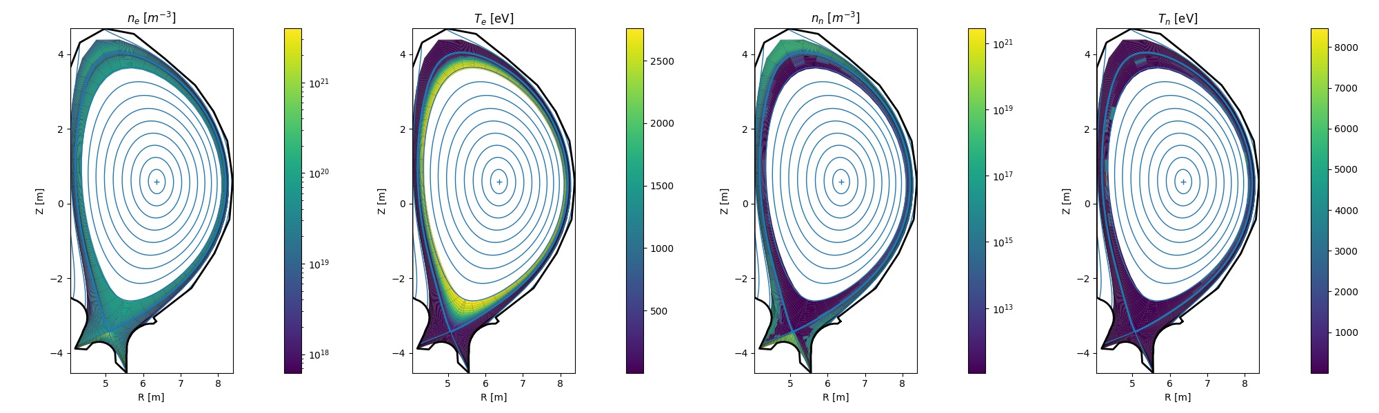
Example of electron density and temperature + atomic D/T neutral density and temperature from a SOLPS-ITER simulation of ITER

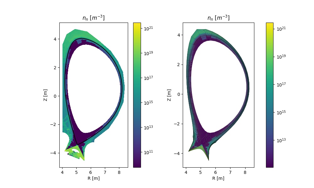
Comparison of D/T atomic neutral density on the B2 and EIRENE grids.

Aurora capabilities to post-process SOLPS results can be useful, for example, to assess synthetic diagnostics for the edge of a fusion device. For this purpose, the eval_LOS() method can help to extract a specific data field from the loaded SOLPS case, interpolating resuls along a line-of-sight (LOS) that goes between two spatial (3D) points. This, combined with Aurora’s capability to examine and simulate atomic spectra, reduces the technical barrier to investigate edge physics.

Interfacing with OEDGE

OEDGE is a simulation package developed around DIVIMP, a Monte Carlo impurity transport code for the plasma edge. OEDGE allows one to load plasma backgrounds from either EDGE2D-EIRENE or B2-EIRENE, or to create approximate backgrounds based on Onion-Skin Modeling (OSM) coupled with EIRENE. Use of the OSM-EIRENE scheme is itself an interesting application of OEDGE.

Aurora includes tools to read OEDGE input files and read/postprocess its results. The following code illustrates how one may run an OEDGE simulation, load and postprocess its results in order to evaluate Balmer line A&M components, using the AMJUEL rates from the EIRENE package:

import aurora
import matplotlib.pyplot as plt

plt.ion()

shot = 38996
time_s = 3.5
label = "osm_test"
casename = f"oedge_AUG_{shot}_{int(time_s*1e3)}_{label}"

# set up an OEDGE case
osm = aurora.oedge_case(shot, (t0 + t1) / 2.0, label=label)

# load a specific input file
osm.load_input_file(filepath="/path/to/my/file.d6i")

# possibly modify specific parts of the input file:
osm.inputs["+P01"]["data"] = 22

# update input file
osm.write_input_file(filepath="/path/to/my/file.d6i")

# now run simulation
osm.run(grid_loc="/path/to/my/grid/file.sno")

# once simulation is run, load the output
osm.load_output()

# now, initialize emission calculation
am = aurora.h_am_pecs()

# extract relevant fields from the OEDGE run
ne_m3 = osm.output.read_data_2d("KNBS")
Te_eV = osm.output.read_data_2d("KTEBS")
Ti_eV = osm.output.read_data_2d("KTIBS")
n_H2_m3 = osm.output.read_data_2d("PINMOL")
n_H_m3 = osm.output.read_data_2d("PINATO")

# load all contributions predicted by AMJUEL
cH, cHp, cH2, cH2p, cH2m = am.load_pec(
    ne_m3,
    Te_eV,
    ne_m3,  # ni=ne
    n_H_m3,
    n_H2_m3,
    series="balmer",
    choice="alpha",
    plot=False,
)

fig, axs = plt.subplots(1, 5, figsize=(25, 6), sharex=True)
osm.output.plot_2d(cH, ax=axs[0])
axs[0].set_title("cH")
osm.output.plot_2d(cHp, ax=axs[1])
axs[1].set_title("cHp")
osm.output.plot_2d(cH2, ax=axs[2])
axs[2].set_title("cH2")
osm.output.plot_2d(cH2p, ax=axs[3])
axs[3].set_title("cH2p")
osm.output.plot_2d(cH2m, ax=axs[4])
axs[4].set_title("cH2m")
plt.tight_layout()

Neoclassical transport with FACIT

The FACIT model can be used in Aurora to calculate charge-dependent collisional transport coefficients analytically for the impurity species of interest. FACIT takes kinetic profiles and some magnetic geometry quantities (which shall be described shortly) as inputs, and outputs the collisional diffusion coefficient \(D_z\) [\(m^2/s\)] and convective velocity \(V_z\) [\(m/s]\) which can then be given as an input for run_aurora().

An example of a standalone call to FACIT is provided in aurora/facit.py, from which profiles of the transport coefficients are obtained:

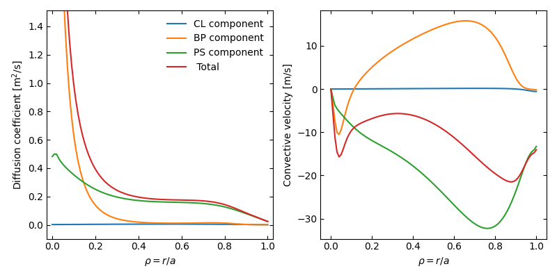
Example of neoclassical W transport coefficients calculated with FACIT.

A complete description of the inputs and outputs of the model is provided in the documentation of the FACIT class.

Note that FACIT provides the individual Pfirsch-Schüter, Banana-Plateau and classical collisional flux components, facilitating additional analysis of the physical processes involved in the transport.

An important feature of FACIT is the description of the effects of rotation on neoclassical transport across collisionality regimes, particularly relevant when heavy impurities like tungsten are analyzed. Rotation is described by the main ion Mach number \(M_i(r) = v_\varphi/v_{ti} = \Omega R_0/\sqrt{2 T_i/m_i}\) and the rotation_model flag. These effects can typically be ignored for light impurities (from experience, the impact of rotation on Argon is small but potentially non-negligible).

Warning

If rotation_model=2, then the flux surface contours \(R(r,\theta)\), \(Z(r,\theta)\) that are inputs of FACIT should have a radial discretization equal to the rho coordinate in which FACIT will be evaluated. If they are not given as inputs, circular geometry will be assumed internally.

A full example on how to run FACIT in Aurora is given examples/facit_basic.py. The following code shows the initialization of the transport coefficients, the magnetic geometry and the main call to FACIT looped over each charge state of the impurity species::

# note that to be able to give charge-dependent Dz and Vz,
# one has to give also time dependence (see documentation of aurora.core.run_aurora())

times_DV = np.array([0])
# note that to be able to give charge-dependent Dz and Vz,
# one has to give also time dependence (see documentation of aurora.core.run_aurora()),
# so a dummy time dimension with only one element is introduced here
nz_init  = np.zeros((asim.rvol_grid.size, asim.Z_imp+1))

D_z = np.zeros((asim.rvol_grid.size, times_DV.size, asim.Z_imp+1)) # space, time, nZ
V_z = np.zeros(D_z.shape)

# flux surface contours (when rotation_model = 2)
RV, ZV = aurora.rhoTheta2RZ(geqdsk, rhop, theta, coord_in='rhop', n_line=201)
RV, ZV = RV.T, ZV.T

# call to FACIT for each charge state
for j, tj in enumerate(times_DV):

    for i, zi in enumerate(range(asim.Z_imp + 1)):

        if zi != 0:
            Nz     = nz_init[:idxsep+1,i]*1e6 # in 1/m**3
            gradNz = np.gradient(Nz, roa*amin)

            fct = aurora.FACIT(roa,
                               zi, asim.A_imp,
                               asim.main_ion_Z, asim.main_ion_A,
                               Ti, Ni, Nz, Machi, Zeff,
                               gradTi, gradNi, gradNz,
                               amin/R0, B0, R0, qmag,
                               rotation_model = rotation_model, Te_Ti = TeovTi,
                               RV = RV, ZV = ZV)

            D_z[:idxsep+1,j,i] = fct.Dz*100**2 # convert to cm**2/s
            V_z[:idxsep+1,j,i] = fct.Vconv*100 # convert to cm/s

Warning

FACIT uses lengths in \([m]\), NOT \([cm]\). In particular, input densities should be given in \([m^{-3}]\) and the output transport coefficients Dz and Vconv should be converted back from \([m^2/s]\) and \([m/s]\) to \([cm^2/s]\) and \([cm/s]\), respectively, before passing them to run_aurora().

In addition to the collisional transport coefficients calculated with FACIT, we can add a turbulent component to the total diffusion and convection, imposed by hand as in previous sections of this tutorial. In this example, we fix an approximate position for a pedestal top at \(\rho_{pol} \approx 0.9\), and assume that turbulence is suppresed inside the pedestal::

Dz_an = np.zeros(D_z.shape) # space, time, nZ
Vz_an = np.zeros(D_z.shape)

# estimate pedestal top position and find radial index of separatrix
rped   = 0.90
idxped = np.argmin(np.abs(rped - asim.rhop_grid))
idxsep = np.argmin(np.abs(1.0 - asim.rhop_grid))

# core turbulent transport coefficients
Dz_an[:idxped,:,:] = 1e4  # cm^2/s
Vz_an[:idxped,:,:] = -1e2 # cm/s

# SOL transport coefficients
Dz_an[idxsep:,:,:] = 1e4  # cm^2
Vz_an[idxsep:,:,:] = -1e2 # cm/s

D_z += Dz_an
V_z += Vz_an

Note

FACIT is distributed within Aurora. The following papers contain the derivation of the model: the self-consistent calculation of the Pfirsch-Schlüter flux and the poloidal asymmetries of heavy impurities at high collisionality is given in Maget et al 2022 Plasma Phys. Control. Fusion 64 069501, while the extension to arbitrary collisionality and inclusion of the Banana-Plateau flux in the poloidally-symmetric (non-rotating) limit is obtained in Fajardo et al 2022 Plasma Phys. Control. Fusion 64 055017, and finally the description of the effects of rotation across collisionality regimes is presented in Fajardo et al 2023 Plasma Phys. Control. Fusion 65 035021. Please cite these papers when using FACIT.